CRU : Projects : SO&P : Data : Model Data : HadCM3 : HadCM3 Data

SO&P: HadCM3 Geographic pattern of sea level anomalies

Important notes regarding the HadCM3 data:

Do not redistribute data to others outside the SO&P project.

Hadley Centre will require co-authorship and need to know from the start what analyses you are using the HadCM3 data for. Please contact Simon Tett (see SO&P participants table) and keep him informed.

To ensure collaboration between SO&P partners, please refer to the list of ongoing/planned model-data comparisons. Please contact others who have listed an interest in the same area, to initiate collaboration. To add your planned areas of model-data work to the list, email Tim Osborn.

A small climate drift, unrelated to the external forcings, is present in the HadCM3 simulations. It's significance depends on the region and variable being considered. Simon Tett describes how this should be dealt with, by reference to the HadCM3 control simulation, in this report (not yet available). The HadCM3 control simulation data is not yet available.

Please inform Tim Osborn of any errors that you find in the data.

For important notes regarding the control simulation: click here.

For important notes regarding the nat simulation: click here.

For important notes regarding the all simulation: click here.

For important notes regarding the sealv variable: click here.

Select alternative variable:
slp__ : sst__ : airtm : rlhum : swrad : precp : snowd : soilm : soilt : win10 : z850_ : z500_ : u500_ : v500_ : iceco : iceth : lwrad : sealv

Select alternative spatial average:
Global : NH : SH : N-extratropics : Tropics : S-extratropics : (or change variable)

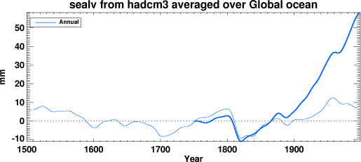
HadCM3 Geographic pattern of sea level anomalies Global (mm)

Ocean (thin lines "nat", thick lines "all", 30-year smoothing, anomalies from 1500-1749 of "nat")	Figures	Data
	hadcm3_sealv_gloocean.gif hadcm3_sealv_gloocean.ps hadcm3_sealv_gloocean.pdf	Annual control nat all

Select alternative spatial average:
Global : NH : SH : N-extratropics : Tropics : S-extratropics : (or change variable)

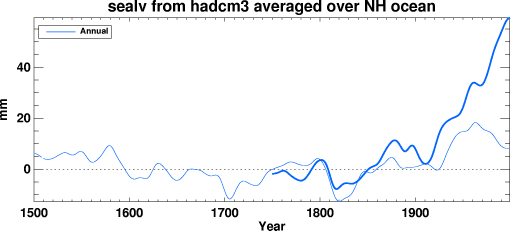
HadCM3 Geographic pattern of sea level anomalies NH (mm)

Ocean (thin lines "nat", thick lines "all", 30-year smoothing, anomalies from 1500-1749 of "nat")	Figures	Data
	hadcm3_sealv_nhmocean.gif hadcm3_sealv_nhmocean.ps hadcm3_sealv_nhmocean.pdf	Annual control nat all

Select alternative spatial average:
Global : NH : SH : N-extratropics : Tropics : S-extratropics : (or change variable)

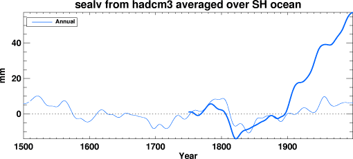
HadCM3 Geographic pattern of sea level anomalies SH (mm)

Ocean (thin lines "nat", thick lines "all", 30-year smoothing, anomalies from 1500-1749 of "nat")	Figures	Data
	hadcm3_sealv_shmocean.gif hadcm3_sealv_shmocean.ps hadcm3_sealv_shmocean.pdf	Annual control nat all

Select alternative spatial average:
Global : NH : SH : N-extratropics : Tropics : S-extratropics : (or change variable)

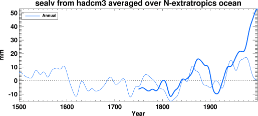
HadCM3 Geographic pattern of sea level anomalies N-extratropics (mm)

Ocean (thin lines "nat", thick lines "all", 30-year smoothing, anomalies from 1500-1749 of "nat")	Figures	Data
	hadcm3_sealv_nexocean.gif hadcm3_sealv_nexocean.ps hadcm3_sealv_nexocean.pdf	Annual control nat all

Select alternative spatial average:
Global : NH : SH : N-extratropics : Tropics : S-extratropics : (or change variable)

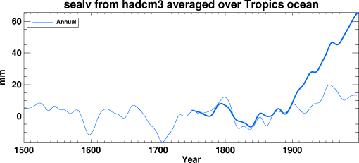
HadCM3 Geographic pattern of sea level anomalies Tropics (mm)

Ocean (thin lines "nat", thick lines "all", 30-year smoothing, anomalies from 1500-1749 of "nat")	Figures	Data
	hadcm3_sealv_troocean.gif hadcm3_sealv_troocean.ps hadcm3_sealv_troocean.pdf	Annual control nat all

Select alternative spatial average:
Global : NH : SH : N-extratropics : Tropics : S-extratropics : (or change variable)

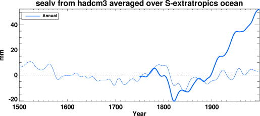
HadCM3 Geographic pattern of sea level anomalies S-extratropics (mm)

Ocean (thin lines "nat", thick lines "all", 30-year smoothing, anomalies from 1500-1749 of "nat")	Figures	Data
	hadcm3_sealv_sexocean.gif hadcm3_sealv_sexocean.ps hadcm3_sealv_sexocean.pdf	Annual control nat all

Important notes regarding the 'control' simulation:

The 'control' simulation has constant external forcings, representative of (approximately) pre-industrial conditions (though, for example, the vegetation cover is set to present day).
In the SO&P web archive we have 1010 years of data from the 'control' simulation. The 'control' simulation actually began 750 years earlier, so essentially we have years 751 to 1760 of the simulation (these are not calendar years!). Even at this stage in the simulation, there are some residual climate drifts (trends) in certain variables.

What does the "year" in the control simulation mean? In the actual netCDF data files provided by the Hadley Centre, the first year of the 'control' run was given the year nominal year "1530", and so the years 751 to 1760 that we have are given nominal years "2280" to "3289". The 'nat' simulation was started from the 1000th year of the 'control' simulation (nominal year "2529" in the netCDF files). The 'nat' simulation is associated with specific calendar years (because the time series of external forcings represents calendar years 1492-1999). Therefore, to compare the 'nat' run with the 'control' run, we need to compare calendar years 1492-1999 with 'control' run nominal years "2529"-"3036" (in fact, in SO&P we are using calendar years 1500-1999, which can be compared with 'control' run nominal years "2537"-"3036"). The 'all' simulation begins in calendar year 1750, and because it starts from the calendar year 1750 conditions of the 'nat' run, its relationship with the control run is the same (i.e., calendar years 1750-1999 should be compared with 'control' run nominal years "2787"-"3036"). The following table may help:

Year conversions	nominal year in netCDF files	year of the control run	corresponding calendar year of nat/all runs
start of control run	"1530"	1	N/A
start of control run data held by SO&P	"2280"	751	1243 AD
start of nat run	"2529"	1000	1492 AD
start of nat run data used by SO&P	"2537"	1008	1500 AD
start of all run	"2787"	1258	1750 AD
end of nat and all runs	"3036"	1507	1999 AD
end of control run data held by SO&P	"3289"	1760	2252 AD

To simplify things, just subtract 1037 from the nominal year stored in the 'control' run data files to convert it to a calendar year for comparison with the 'nat' and 'all' simulations. In the time series files this has already been done.

Important notes regarding the 'nat' simulation:

The surface roughness due to vegetation cover was incorrectly set to present-day, rather than pre-industrial, values during this simulation. This results in a step-change between this 'nat' simulation and the 'all' simulation in 1750 (because the vegetation roughness is changed to pre-industrial cover at the start of the 'all' simulation). Simon Tett will be calculating some correction fields for each variable, which can be applied to the 'nat' simulation data to remove the vegetation error effects.
The data files run from 1492-1999, but in SO&P we are using data from 1500-1999 only.

Important notes regarding the 'all' simulation:

The vegetation cover was incorrectly set to present-day, rather than pre-industrial, during the 'nat' simulation. The 'all' simulation should start smoothly from the 'nat' simulation in 1750, but because of the sudden change from present-day to 1750 vegetation there is a step-change between the two simulations. Simon Tett will be calculating some correction fields for each variable, which can be applied to the 'nat' simulation data to remove the vegetation error effects.
The stratospheric ozone depletion used as a forcing in the 'all' simulation was too strong by a factor of around 2. This may affect some variables (e.g. Antarctic atmospheric circulation) in the final 3 decades of the simulation. Simon Tett is considering a re-run of these final decades.

Important notes regarding the sealv variable:

It is extremely important to realise that the sealv variable does not contain the correct global-mean changes.

The global-mean of the sealv data from any one year should be calculated (using area-weighting of each grid cell, which is proportional to the cosine of the latitude of the cell) and subtracted from the sea level at every individual grid cell for the same year. This will yield patterns of local sea level deviations from the global-mean for that year.
To obtain the actual simulated local sea levels, the correct global-mean value of sea level for the year (see HadCM3 global-mean sea level) should be added to the pattern of local sea level deviations.
By adding the sum of (1) the global ocean expansion and (2) the global glacier/small-ice-cap melt component, then the local sea levels will capture both components plus the local deviations from this.
Note also that the absolute values are arbitrary (there is no definition of "zero" sea level) and so some adjustment to a common baseline period is necessary before comparing different regions and/or different model simulations.
- A suggested adjustment is this: after combining the local and global changes as described above, subsequently add a constant to each grid cell's sea level time series so that it has zero mean over the 1500-1549 period in the 'nat' simulation. For the 'all' simulation, add a constant to each grid cell's sea level time series so that it has the same mean as the adjusted 'nat' series over the 1750-1799 period.

Last updated: August 2004, Tim Osborn