Simple climate models for teaching

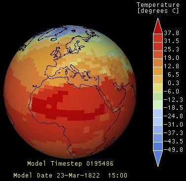This set of webpages brings together a number of resources that may prove useful for incorporating exercises with computer-based climate models into climate science teaching.

The focus is on masters-level teaching, but for our MSc in Climate Change the students have such a wide range of natural and social science backgrounds that we offer no formal practical classes where climate models are used in great depth. Most of the material presented here does not require high levels of quantitative or computer skills, and may well prove useful for teaching purposes at a range of different levels.

Acknowledgements and limitations for using this material

Most of these climate model resources are already available on the web, and I have simply made a selection from the wide variety of models that are available, added some comments, and in some cases suggested some exercises that might be undertaken using these models. The providers of these resources are gratefully acknowledged.

I have, however, developed some new content for these webpages; principally, the simple spreadsheet-based global-climate model and some of the suggested exercises. You are welcome to make use of these, but it would be nice if you acknowledged me as the source when doing so.

If you make any improvements or extensions, then I would be happy to hear about them. My contact details are on my homepage. However, please don't ask me to make improvements or extensions, as I just don't have the time.

1. Introduction to climate modelling

   An obvious question that ought to be asked first is, why do we need climate models? There are three principal reasons: (1) to better understand climate system behaviour, (2) to explore the causes of past climate change, and (3) to make predictions of possible future climate change.

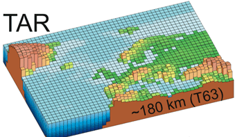
   The second question to consider is, what is a climate model? Models are simplifications of reality. As such, we should never replace observations of the real system by predictions from a simplified model, nor should we expect models to be able to perfectly reproduce reality. Simplifications may be made in a number of ways. We could omit some dimensions. Or we could include a dimension but with limited detail (often called the "resolution" of the model, with coarser resolution providing less detail -- see figure). We could omit some processes. Or we could make a simplified approximation to some complex process (often called a "parameterisation"). But we must retain sufficient detail to capture the essence of the system and its behaviour for the application at hand.

   Climate models are mathematical representations of the climate system based on physical principles, usually solved on a computer. There are many types of climate model, ranging from energy balance models to Earth system models. Currently, the most widely used climate models consist of a three-dimensional "General Circulation Model" (GCM) of the atmosphere coupled to a three dimensional model of the ocean, and including models of sea ice and land surface conditions.

   An extensive introduction to climate system processes is given by Harvey (2000), and a widely used primer on climate modelling is that of McGuffie and Henderson-Sellers (1997).

2. Understanding climate system behaviour: simple energy balance models

   Simple energy balance models typically simulate just the global-average energy budget of the Earth, which is dominated by the balance between incoming solar radiation and outgoing terrestrial radiation. Non-radiative transfers from the surface to the atmosphere must also be included if the model is to get the correct absolute surface temperature, but some models only attempt to simulate perturbations (i.e. changes) in temperature in response to a change in the radiative balance, and these do not need to explicitly represent the non-radiative transfers. The key components of the Earth's energy balance and how these can be represented in simple climate models are described in my lectures (available at the UEA Portal/Blackboard site for the Science of Climate Change module). Other, more detailed descriptions of the history of radiation balance calculations and the derivation of more realistic, yet still relatively simple, energy balance models are available (those linked here are just examples).

   • The model: simple spreadsheet climate model (this is a Microsoft Excel spreadsheet file)
     • Developed by Tim Osborn (homepage).
     • The spreadsheet equations represent a global-mean energy balance model consisting of a surface temperature and an ocean temperature. The ocean covers 70% of the Earth's surface (the remaining 30% is assumed to have zero heat capacity) and is represented by two completely-mixed boxes (the upper and mid-depth ocean; the deep ocean is not represented). The model is a perturbation model, simulating the change in temperature driven by a given change in forcing. If forcing is set to zero, the temperature perturbation will eventually also reach zero.

   • General instructions:
     • The spreadsheet is "protected" so that you can only alter the values in the cells highlighted by orange shading. There are two sets of these orange input values. In column D, rows 16 to 21, there are six model parameters (e.g. the climate sensitivity of the model), while in rows 26 to 28, columns J to Y, are eight factors that control the forcing time series that is applied to the model.

       The model inputs and outputs are shown in the three graphs. The forcing chosen for each experiment is shown by the green line in the upper graph. The lower two graphs show the simulated temperature (in green) for individual yearly values (left) and for decadally-smoothed values (right). These graphs also include (in pink) the observed global-mean temperature, which provides a useful comparison for some simulation experiments.

       Each experiment requires a forcing time series to be generated. The forcing is composed of a sum of individual forcing components (estimates of volcanic, solar, greenhouse gas and tropospheric sulphate aerosol forcings from 1765 to 2006 are provided), each multiplied by a factor that the user chooses via the orange boxes. To turn off a particularl forcing, simply set that forcing factor to zero. A guideline range is given for each forcing factor, based loosely on the uncertainty estimated by the IPCC.

       There are also two further forcing components that can be included (by setting their factors to a positive, non-zero value). First is a random component to generate the temperature fluctuations that are not driven by external forcings but instead arise through internally-generated variability. Because this simple energy-balance model does not generate internal weather variability, it is necessary to using a random forcing term as a substitute. 100 different random sequences are provided, which can be selected by entering a value between 1 and 100 in cell M28. Second is a sinusoid (sine-wave) forcing, for which the amplitude and period can be chosen. This is useful for exploring the behaviour of the climate model to forcings with different time scales.

   • Exercise:
     • The suggested exercises are described in this PDF document: simple_climate_model_exercises.pdf. There are two "sensitivity experiments" that are designed to explore the behaviour of the climate system, particularly how the climate responds differently to forcings that last either a short or a long time. The other three "simulation experiments" are various attempts to simulate the changes in global temperature that have been observed over the last 150 years.

   • Hints and outcome:
     • Hints and learning outcomes for these five exercises are described in this PDF document: outcome_simple_climate_model_exercises.pdf.

3. Forcing factors that drive climate change

   There are a range of drivers (or forcings) of climate change, including both natural and anthropogenic forcings. Some of these are simply known or estimated from observations -- e.g. the atmospheric concentration of CO₂ over recent decades or centuries. However, there are a few forcing factors that can be predicted using models that describe the processes that drive the forcings.

   I have selected two forcing factors for further experimentation:

   • Orbital forcing of climate

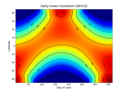     On very long time scales (10s to 100s of thousands of years), the sequence of glacial and inter-glacial periods that the Earth has exhibited during the last few million years are considered to have been driven by semi-regular wobbles in the orbit of the Earth around the sun. These Milankovitch cycles alter the total solar insolation received at the top of the Earth's atmosphere -- and, most importantly, the seasonal and geographical distribution of the insolation. In particular, the amount of summer insolation at mid-to-high latitudes of the Northern Hemisphere is considered to be important in determining whether snow/ice melts during summer or is able to survive the summer and eventually accumulate into large ice sheets.

     • The model: orbital forcing of climate
       • Provided by David Archer, in association with his book, Archer (2006).

     • General instructions:
       • Click the link above for a brief overview of the model. You then have two choices.

         "Snapshot" generates a latitude-longitude map of solar insolation received at the top of the Earth's atmosphere for a selected year. Try this out, perhaps comparing the pattern for the present day (2009) with that for 6000 years before present (-4000). The differences may not appear large, but bear in mind that the contour interval is 100 Wm^-2: compare this to the global-mean forcing of 3.7 Wm^-2 due to a doubling CO₂ concentration. A further point to note is that this model predicts solar insolation at the top of the atmosphere, which peaks near the poles during summer time due to the long polar days. The actual energy absorbed by the climate system or the solar insolation received at the surface peaks in the tropics, because the reflection of insolation by clouds and by the Earth's surface (particularly when covered in snow or ice) tends to be greater at higher latitudes. Take a look at the first figure on the Insolation page at Wikipedia to see the difference the atmosphere and surface make to the insolation received.

         "Time series" is the second choice, creating a graph of the past and/or future time evolution of solar insolation, at each latitude, but for only one time of the year.

     • Exercise:
       • Use the "time series" option to investigate when the next ice age glaciation might be triggered by a big reduction in summer insolation received at mid-to-high latitudes of the Northern Hemisphere. How far in the future does such a reduction next occur?

     • Hints and outcome:
       • Use the "time series" option, choose day 180 (day 1 is 1st January, so day 180 is in the Northern Hemsphere summer -- it's actually 29th June) and a range from -4000 (which is 4000 BC, or 6000 years before present) through to 60000 (sixty thousand years AD!). Look at the changes in the mid-to-high northern latitudes (e.g. at 65N). There are some fluctuations, but it may be hard to see any big decreases.

         Instead, you can inspect the data values themselves: click the link to "pick up the data". This shows the data for all latitudes and all times, as a text file. Far too big to examine fully. But if you do an automatic search for "-65" (note that there is an error in this model output, which records 65N as -65 rather than +65) you can fairly quickly scan through the insolation values at 65N, watching how they vary with time (in most browsers or text viewers you can do this with shortcut keys or mouse clicks; e.g. <ctrl>F to find the first "-65" and then repeatedly press <ctrl>G to jump to each subsequent occurrence).

         You should find that insolation was over 500 Wm^-2 at 6000 BP (year -4000 in the file), during the "Holocene Climate Optimum", reducing to 476.9 W^-2 by the present day (year 2016 is the closest to the present day in the model output). It then stays within the range 475 to 502 Wm^-2 until 52,000 AD, before dropping to a minimum of 467 Wm^-2 in 56,032 AD. If summer insolation at 65N needs to fall below its present-day value to initiate the next ice-age glaciation, then the next glaciation is at least 50,000 years away.

   • Greenhouse gas forcing in the 21st century

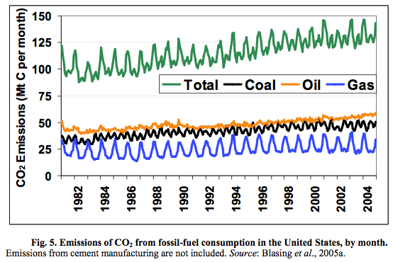     The emissions of the CO₂ and other greenhouse gases by human activity can be predicted by the Kaya identity, developed by Japanese economist Yoichi Kaya. The Kaya identity and similar approaches have been used to generate many of the commonly used greenhouse gas emissions scenarios, including the IPCC SRES scenarios.

     The Kaya identity states that emissions of CO₂ are the product of four inputs: population, GDP per capita, energy consumed per unit of GDP, and carbon emissions per unit of energy consumed. The future evolution of these four terms must be estimated (from assumptions about demographic, economic, technological and societal change) to generate the emissions scenario.

     • The model: Kaya identity
       • Provided by David Archer, in association with his book, Archer (2006).

     • General instructions:
       • Click "run me" to open the Kaya identity model page. The page displays the equation of the Kaya identity. The identity itself is fairly simple -- it is "predicting" the four input terms that is difficult. This model allows you to explore these by varying four assumptions about how each of the input terms may change in the future. Either use the default values, or enter your own estimates, and click "do the math" to generate the model's output.

         The model produces seven output plots. The last four are the four input terms: population, GDP per capita, energy consumed per unit of GDP (energy intensity), and carbon emissions per unit of energy consumed (carbon efficiency). You can alter the rate at which these various terms change and see how they match the observed trends up to 2000 (indicated by the + symbols).

         The first plot shows are the output of the Kaya identity in terms of global anthropogenic carbon emissions (historical estimates are again indicated by the + symbols).

         The second and third plots are useful for exploring the implications for stabilising atmospheric concentrations of CO₂ are various levels. The CO₂ concentrations that might result from the predicted carbon emissions (according to one particular carbon cycle model, the ISAM model) are shown in red in the second plot, compared with various alternative evolutions that lead to concentrations stabilising at various levels from 350 to 750 ppm. The third plot indicates the additional carbon-free energy required to bring your particular scenario on to a path that stabilises at various levels from 350 to 750 ppm (if your scenario is already lower than some of the stabilisation pathways, then the third plot will show negative values, indicating that we could actually emit more carbon and still reach a particular stabilisation target). Watch out(!), the colours used for each line in panels 2 and 3 do not match, and also the 750 ppm stabilisaton line in panel 2 is hard to see, as it's yellow on a white background.

     • Exercise:
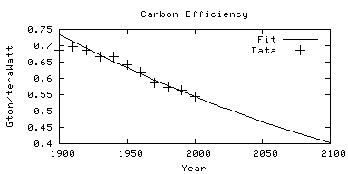       • Typically, population and wealth are expected to show long-term growth, while the energy needed to support this economic growth and the carbon emitted in generating the energy are expected to show relative declines. For most scenarios, and certainly for the default values, the population and economic growth exceed the reductions in energy intensity and carbon efficiency, resulting in continuing growth of emissions and CO₂ concentrations that do not begin to stabilise during the 21st century.

         The EU's target is to avoid global temperatures rising more than 2 degrees C above pre-industrial levels, a target which could perhaps be achieved (though not definitely, because it depends how sensitive the climate is) if the total greenhouse-gas forcing is equivalent to 450 ppm of CO₂ or lower. Suppose the world population levels out at 9 billion, GDP per person grows at 1.6 %/yr, while energy intensity reduces at -1 %yr. How fast must carbon efficiency fall if the EU's target is to be met?

     • Hints and outcome:
       • Set the "population levels out at" box to 9 (billion), GDP/person growth to 1.6 %/yr, and energy intensity change to -1 %/yr. Vary the carbon efficiency until the CO₂ concentration in the second panel stays below 450 ppm.

         A reduction of -2.1 %/yr in carbon efficiency achieves the target of keeping CO₂ from exceeding 450 ppm. Such a reduction would lower the carbon emitted per Terawatt of energy generated from 0.55 Gton in 2000 to 0.07 Gton in 2100, almost a tenfold reduction, perhaps quite a challenging target? Note also that the target really requires CO₂ to be stabilised below 450 ppm to allow for some increases of the other greenhouse gases.

4. General circulation modelling

   The EdGCM (Educational Global Climate Modelling) project (see http://edgcm.columbia.edu/) have developed a GCM-based climate model with a user-friendly interface that runs on desktop computers. It can be installed on either Windows or MacOS systems, and comes with a range of analysis and visualisation tools. Also included in the package are surface boundary condition data and forcing data to allow users to make a number of GCM experiments simulating either past or future climate changes.

   • The model: EdGCM (this is a website from where the model can be downloaded and installed)
     • Developed by the EdGCM team at Columbia University and NASA's Goddard Institute for Space Studies
     • The EdGCM model is similar to the coarse-resolution GISS climate model from around 1990, but with a new user interace for setting up, running, and analysing GCM experiments. The aim is that research-quality GCM experiments could be undertaken by university-level students; there is technical support, a community forum for exchanging results and solutions to problems, and materials for educational exercises. One thing to bear in mind when using EdGCM is that this GCM has quite a high equilibrium climate sensitivity (around 5 degC for a doubling of [CO₂]), which is outside the likely range of values reported by the IPCC.

   • General instructions and exercises:
     • The instructions for downloading, installing and running EdGCM are provided at the EdGCM website. I was able to complete the task and begin a first, test simulation with EdGCM after 1 to 2 hours of work, and there is a forum where you can ask questions if you get stuck.

       I have not set any specific exercises to complete with EdGCM. Again, the EdGCM software, website and instruction manual provide a range of suggested experiments and information on how to set them up. Good luck!

   • Other GCM-based climate models:
     • There are a number of other GCM-based climate models that are freely available for academic or personal research use. These models are closer to the "start-of-the-art" than EdGCM, but they do not necessarily have the ease of use, community support or other elements that lend themselves to educational use that the EdGCM project provides. As such, they would require considerably more effort to master the initial phases of learning to use them.
       
       
       • Community Climate System Model (e.g. NCAR CCSM 3.0): Support & Model code
         
         
       • Goddard Institute for Space Studies (GISS Model E): Support & Model code
         
         
       • Met Office Hadley Centre "Unified Model" (e.g. HadCM3, HadGEM1): Support & Model code
         
         
     • You may also be interested in the climateprediction.net experiment. This allows you to participate in a distributed computing experiment using the Met Office Hadley Centre's GCM-based climate models, which has so far (as of August 2009) completed around 45 million years of climate simulation. Participating in this project does not allow you to design your own experiments, but they do provide a description of the experiments that you will perform, and scientific papers based on the results.

5. Exploring possible future climate change

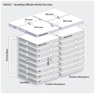   There are a number of tools to make predictions of future climate change (especially in terms of global-mean temperature change). I have selected two tools that may be particularly useful or relevant, especially to MSc dissertation projects that focus on global or UK climate changes. The first is the simple climate model MAGICC, which can be installed on Windows systems, and has an easy-to-use graphical user interface that allows you to explore uncertainty in predictions of global temperature change and how various climate policy options may mitigate the magnitude of future changes. MAGICC is also coupled to SCENGEN, which uses patterns from existing GCM experiments to estimate possible regional climate changes from the MAGICC-simulated global temperature change. The second tool is the UK Climate Projections 2009 (UKCP09) portal. This is a web-based interface (so it does not need installing on your computer) that allows access to the UKCP09 projections of future UK climate change. No specific exercises have been developed for either of these tools at present. Just try them out and see what you can learn!

   • The model: MAGICC/SCENGEN version 5.3 (this is a website from where the model can be downloaded and installed)
     • Developed by Tom Wigley and Sarah Raper (with additional input from a number of others)

   • General instructions and exercises:
     • The MAGICC/SCENGEN website contains a link to a user manual. As a first exercise, simply follow the sequence of steps that is illustrated on pages 21-35 of the MAGICC/SCENGEN user manual. This exercise leads you through the process of showing CO₂ concentration, global temperature and global sea level for an SRES scenario compared with a scenario that stabilises at 450 ppm of CO₂ concentration, and how this is influenced by carbon cycle feedbacks and climate sensitivity uncertainty.
   • The tool: UK Climate Projections 2009
     • Developed by the Met Office Hadley Centre, UK Climate Impacts Programme, and other partners.

   • General instructions and exercises:
     • UKCP09 combines a number of consistent resources: reports, maps, interactive web pages and a weather generator.
       
       
       • UKCP09 reports and publications: try the "Briefing Report" for an initial overview, before reading others if you want further details.
         
         
       • UKCP09 pre-prepared maps & graphs: view maps for a range of variables (seasonal temperature, precipitation, etc.), under different emissions scenarios, and also showing the probability ranges that take into account many of the uncertainties associated with making projections of possible future climate.
         
         
       • UKCP09 user interface: allows access to the interactive part of UKCP09 and the weather generator (for generating plausible sequences of weather under different future scenarios). You need to register (for free) before using this part of UKCP09, but the process is very simple.
         • Suggested exercise: make a 2D probability plot, showing the probability of summer temperature and summer rainfall changes for Norwich, under the medium (SRES A1B) emissions scenario, for the 2080s.
         • Hints: go to UKCP09 user interface (see above) and choose options in this order: "Start a new request", "by selecting Data source", "Next", "UK Probabilistic Projections of Climate Change over Land", "Future Climate Change Only", then tick both "Change in mean temperature" and "Change in precipitation", "Next", "Medium", "Next", then tick "2080s (2070-2099)" and "Summer (JJA)", "Next". You now should have map to choose your location. You could zoom in and click the square that contains Norwich or type "Norwich" and then click "Search". Either way, you should end up with Grid Cell Id 1477, and then click "Next". Choose "Sampled data", "Select All", "Next", "Joint Probability Plot", and finally "Next". After around 30 seconds, you should be presented with the results, as shown in the figure.

           

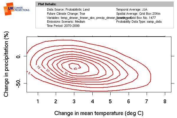
         • These results indicate that the most likely change is about 3 degC of warming and a 20% decrease in rainfall, but that the probability range (based on uncertainties in predicting future global and regional climate change) spans from less than 1 degC to 7 degC, and from a 20% increase to a 60% decrease in rainfall.

Glossary

Anthropogenic

Arising from human activity.

BP

Years Before Present (6000 BP is 6000 years before present, or about 4000 BC).

GCM

General Circulation Model (sometimes used for Global Climate Model).

Insolation

The amount of solar radiation received in a given time (be careful to note whether the insolation at the top of the atmosphere or at the Earth's surface is being described; the latter will be reduced through reflection and absorption by clouds and the atmosphere).

IPCC

Intergovernmental Panel on Climate Change.

MAGICC

A Model for the Assessment of Greenhouse gas Induced Climate Change (an energy balance, upwelling-diffusion climate model developed by Wigley, Raper and Meinhausen).

SRES scenarios

The scenarios of possible future greenhouse gas emissions reported in the IPCC's Special Report on Emissions Scenarios (SRES), published in 2000.

References

• Archer D (2006) Global warming: understanding the forecast. Wiley-Blackwell, 288pp.
• Harvey LDD (2000) Global warming: the hard science. Pearson, Harlow, UK, 336pp.
• McGuffie K and Henderson-Sellers A (1997) A climate modelling primer (2nd edition). Wiley, Chichester, UK, 253pp.

Footnote

This web-based resource was developed for Module 3 [School/discipline-based practice (I)] of my Postgraduate Certificate in Higher Education Practice, during academic year 2008-9. Many thanks to the staff and students who made useful comments and suggestions during the development of this resource.