Hemispheric and global averages graph
(also available as a PDF)
More graphs below and here
|
Hemispheric and global averages graph (also available as a PDF) More graphs below and here |
HadCRUT is a global temperature dataset, providing gridded temperature anomalies across the world as well as averages for the hemispheres and the globe as a whole. CRUTEM and HadSST are temperature datasets for the land and ocean regions, respectively, and contribute to the global dataset.
New versions HadCRUT5 and CRUTEM5 were published in December 2020 (see Morice et al. (2021) and Osborn et al. (2021). The compilation of land air temperature records now includes more stations, and biases in sea surface temperature observations have been reduced. Improved methods of analysis and gridding extend the spatial coverage and reduce coverage biases and reduce uncertainty, especially in the period since 1960.
For the land dataset, there are now two versions:
For the global land and ocean dataset, there are also now two versions:
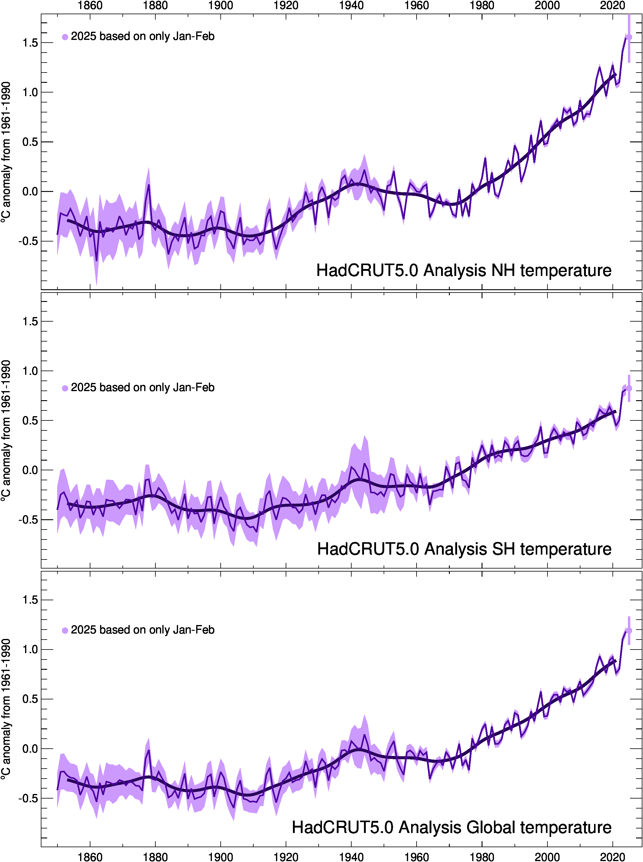
For our best estimate of how global temperature has changed since 1850, we recommend you use the HadCRUT5 Analysis.
The latest version is HadCRUT5, formed using data from CRUTEM5 and HadSST4. All versions are being updated at one or two monthly intervals.
For all versions, hemispheric and global averages as monthly and annual values are available as separate files, alongside the gridded monthly data.
These datasets have been developed by the Climatic Research Unit (University of East Anglia and NCAS) jointly with the Hadley Centre (UK Met Office), apart from the sea surface temperature (SST) dataset which was developed solely by the Hadley Centre.
This webpage gives some brief information to users about the datasets including:
CRU gratefully acknowledges the long-term support for developing, improving and updating these datasets provided by the US Department of Energy (1984-2014) and by the UK National Centre for Atmospheric Science (NCAS) (2016-present), a NERC collaborative centre.
Additional support is also acknowledged: CRUTEM5.0 and HadCRUT5.0 were partially supported by NERC through both the SMURPHS (grant NE/N006348/1) and GloSAT (grant NE/S015582/1) projects.
The Met Office component of this work is supported by UK BEIS and Defra, through the Hadley Centre Climate Programme.
| Dataset Version |
End month Updated |
Grid | Hemispheric & global means CRU format text files |
Station data | CEDA or Met Office For more data files including uncertainties |
|||||||
|---|---|---|---|---|---|---|---|---|---|---|---|---|
| HadCRUT5 Analysis version 5.0.2.0 |
2024-05 2024-07-08 | netCDF (21MB) |
|
Same as CRUTEM5 | Met Office: HadCRUT5 CEDA (not updated): HadCRUT5 |
|||||||
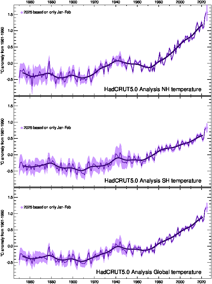
| Combined land [CRUTEM5] and marine [HadSST4] temperature anomalies on a 5° by 5° grid with greater geographical coverage via statistical infilling (Morice et al., 2021) | ||||||||||||
| HadCRUT5 Non-Infilled version 5.0.2.0 |
2024-05 2024-07-08 | netCDF (21MB) |
|
Same as CRUTEM5 | Met Office: HadCRUT5 CEDA (not updated): HadCRUT5 |
|||||||
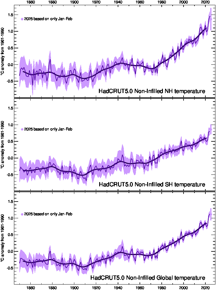
| Combined land [CRUTEM5] and marine [HadSST4] temperature anomalies on a 5° by 5° grid with geographical coverage limited to grid cells close to where we have measurements (Morice et al., 2021) | ||||||||||||
| CRUTEM5 version 5.0.2.0 |
2024-05 2024-07-08 | netCDF (21MB) |
|
Text stations (gzip) CRU format Station normals Station SDs format netCDF stations (zip) |
Met Office: CRUTEM5 CEDA (not updated): CRUTEM5 |
|||||||
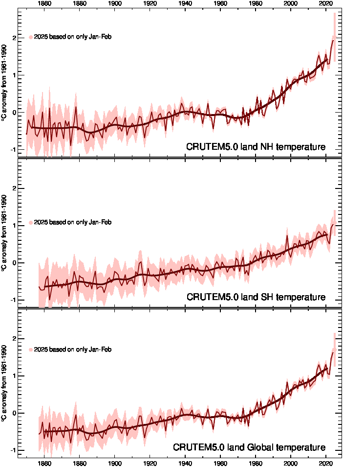
| Land air temperature anomalies on a 5° by 5° grid, not infilled (Osborn et al., 2021) | ||||||||||||
| CRUTEM5alt version 5.0.2.0 |
2024-05 2024-07-08 | netCDF (21MB) |
|
Same as CRUTEM5 | Met Office: CRUTEM5 | |||||||
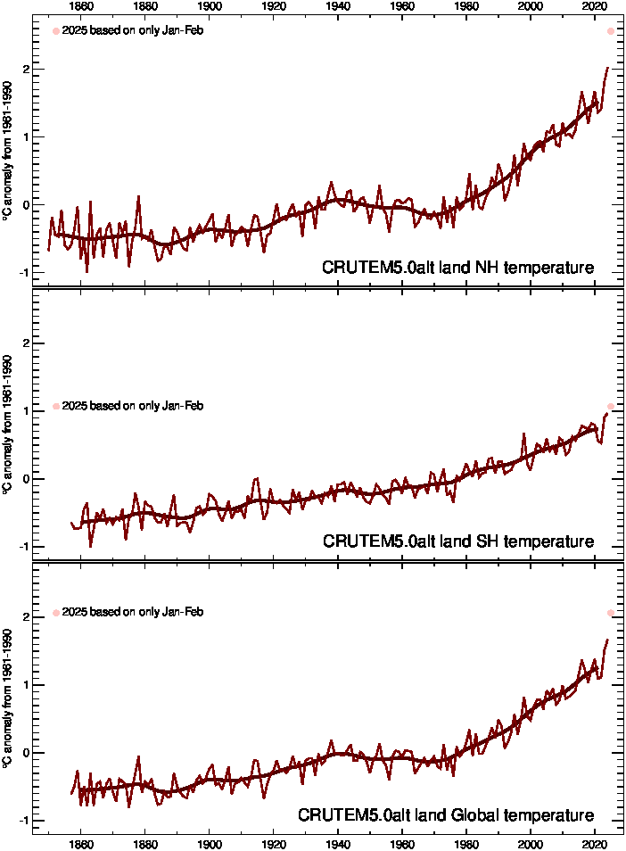
| Land air temperature anomalies on a 5° by 5° grid, not infilled but with better representation of high-latitude stations (Osborn et al., 2021) | ||||||||||||
| HadSST4 version 4.0.1.0 |
2024-05 2024-07-08 | netCDF (21MB) |
|
Not applicable | Met Office: HadSST4 | |||||||
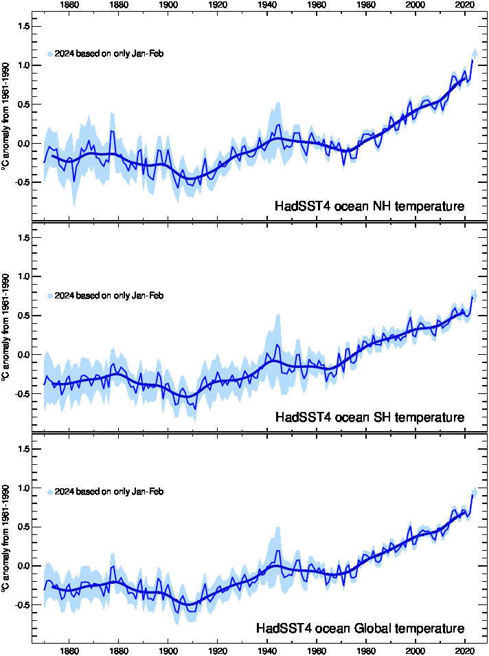
| Sea surface temperature anomalies on a 5° by 5° grid (Kennedy et al., 2019) | ||||||||||||
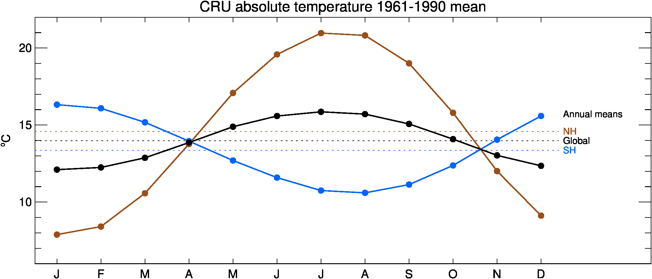
| Absolute 1961-1990 mean | Static | netCDF (<1MB) |
|
Not applicable | Not applicable | |||||||
| Absolute temperatures for the base period 1961-90 on a 5° by 5° grid (Jones et al., 1999). Note that in this file, latitudes run from South to North to match the HadCRUT5 gridded files (in contrast to the absolute temperature file supplied with HadCRUT4). | ||||||||||||
| Hemispheric/global average data file format |
|---|
for year = 1850 to endyear format(i5,13f7.3) year, 12 * monthly values, annual value format(i5,12i7) year, 12 * percentage coverage of hemisphere or globe |
|
Coverage of 0 means data not yet available
Download an R function to read this format |
Timeseries of global and hemispheric mean temperature anomalies as well as maps of the current year's data are available here. These have now been updated to use HadCRUT5 and CRUTEM5.
Also see Tim Osborn's take on Ed Hawkins' famous temperature spiral.
For graphs (and data) of individual land grid cells or individual weather stations, use our CRUTEM Google Earth interface. WARNING: this currently uses the superseded version CRUTEM4. Check back here when we have updated it to the current CRUTEM5 version.
HadCRUT5 and CRUTEM5 datasets are available for further online analysis at the KNMI Climate Explorer.
Every 1 to 3 years, we also add in updated data for stations that do not report in real time, by using
station data that we access from National Meteorological Services (NMSs) around the
world. These updates typically take place between May and September, as by then sufficient
NMSs should have made their monthly average data available for the preceding year. Where
available, we add in extra data from some NMSs when they make more homogeneous
data available. This includes routine updates from the USA, Canada, Russia, China,
Australia and a number of European countries.
How are the hemispheric and global anomaly series calculated?
Values for the hemisphere are the weighted average of all the non-missing, grid-box
anomalies in each hemisphere. The weights used are the cosines of the central latitudes of
each grid box.
For CRUTEM5, the global average is a weighted average of the Northern Hemisphere (NH) and Southern Hemisphere (SH). The weights are two for the NH and one for the SH, based on the relative areas of land in the two hemispheres. See Osborn and Jones (2014) for how this differs from previous versions of CRUTEM. In the CRUTEM5 timeseries files and graphs above, we only show the SH and global averages from Jan 1857 onwards because the land data coverage in the SH is poor before 1857.
For HadCRUT5, the global average is the unweighted average of the NH and SH values.
In the CRU-format timeseries files, the second row of integers is the
percentage of the surface area covered for each month from 1850.
What are the basic raw data used?
For land regions of the world, timeseries of monthly-mean temperatures were compiled from
over 10,000 weather stations for consideration in CRUTEM5.0. Of these, almost 8,000 were actually
used to produce the gridded CRUTEM5.0 dataset while the remainder were not used because
they did not have sufficient data to estimate a 1961-1990 mean (or "normal").
Coverage is denser over the more populated parts of the world, particularly, the United States,
southern Canada, Europe and Japan. Coverage is sparsest over the interior of the South
American and African continents and over Antarctica. The number of available stations
was small during the 1850s, but increases to over 2,000 stations by 1900 and more than
5,000 stations during most of the 1951-2010 period (see Fig. 8 of Osborn et al., 2021).
Raw station data used to produce CRUTEM5 are available from the table above .
For marine regions, sea surface temperature (SST) measurements taken on board merchant and naval vessels, and in more recent decades from instruments mounted on fixed and drifting buoys. As the majority came from the voluntary observing fleet until the 1980s, coverage is reduced away from the main shipping lanes and over parts of the Southern Ocean.
The development of the CRUTEM5 and HadSST4 datasets is extensively discussed in Osborn
et al. (2021) and Kennedy et al. (2019). Both these sources and references
therein also discuss the
consistency and homogeneity of the measurements through time and the steps that have been made
to remove non-climatic inhomogeneities.
Why are sea surface temperatures rather than air temperatures used over the oceans?
Over the ocean areas the most plentiful and most consistent measurements of temperature
have been taken of the sea surface. Marine air temperatures (MAT) are also measured and would,
ideally, be preferable when combining with land air temperatures, but they involve more
complex problems with homogeneity than SSTs (Kennedy et al., 2019). The problems are
reduced using only night marine air temperature (NMAT) but at the expense of discarding
approximately half the MAT data. Our use of SST anomalies implies that we are tacitly
assuming that the anomalies of SST are in agreement with those of MAT. Kennedy et al.
(2019) provide comparisons of hemispheric and large area averages of SST and NMAT anomalies.
See also the GloSAT project which is developing a
global temperature dataset using air temperature over both the oceans and land.
Why are the temperatures expressed as anomalies from 1961-1990?
Stations on land are at different elevations, and different countries calculate average monthly
temperatures using different methods and formulae. To avoid biases that could result from
these differences, monthly average temperatures are reduced to anomalies from the period with
best coverage (1961-90). For stations to be used, an estimate of the base period average must
be calculated. The average temperature for each calendar month in the base period is called a
"normal". Because many stations do not have complete records for the 1961-90 period
several methods have been developed to estimate 1961-90 averages from neighbouring
records or using other sources of data (see Osborn and Jones, 2014 and references therein).
Over the oceans, where observations are generally made from mobile platforms,
it is impossible to assemble long series of actual temperatures for fixed points. However it is
possible to interpolate historical data to create spatially complete reference climatologies
(averages for 1961-90) so that individual observations can be compared with a local normal
for the given day of the year (more discussion in Kennedy et al., 2019).
It is possible to obtain an absolute temperature series for any area selected, using data from the
absolute file, and then add this to a regional average of anomalies calculated from the gridded
data. If a regional average is required, users should calculate a regional average time series of
anomalies, then average the absolute file for the same region, and lastly add the absolute average
to each of the values in the anomaly time series. Do NOT add the absolute values to every grid box in
each monthly field and then calculate large-scale averages.
Why do anomalies not average exactly zero over 1961-1990?
Not all regions
have complete data for the 1961-1990 period, so the anomaly data do not average exactly to
zero for this 30-year period. This applies to the global and hemispheric average series as
well as the individual grid-box series.
How are the land and marine data combined?
Unlike previous versions, HadCRUT5 is NOT created by merging the separately constructed
grids of SST anomalies in HadSST4 and land air temperature anomalies in CRUTEM5. Instead
these SST and land datasets are used as input to a separate spatial model that represents
a temperature anomaly as a combination of anomalies represented by a Gaussian process with
a simple covariance structure together with a changing global-mean temperature anomaly.
This spatial model takes into account the observational uncertainties that have been
estimated for the SST and land temperature anomalies. This analysis process is applied to
the same field of 5°x5°
latitude/longitude grid cells as the input HadSST4 and CRUTEM5 datasets.
However, because each grid cell anomaly is re-estimated using the above spatial process, they
will usually differ from the anomalies in the input datasets.
The entire process produces an ensemble of 200 realisations which represent the uncertainty that arises from the underlying measurements and in the estimate of the spatial fields from the sample of measurements available.
Two versions are provided: HadCRUT5 Non-Infilled provides values only in grid cells which
contain at least one measurement during the year and month being considered, whereas
HadCRUT5 Analysis extends the values to all grid cells where the underlying measurements
are considered to be informative.
The analysis method is described in Morice et al. (2021).
How accurate are the hemispheric and global averages?
The best estimates -- the mean values of the ensembles -- are provided on this CRU webpage.
The uncertainties in the gridded data are represented by the 200-member HadCRUT5 ensemble, and
for the global and hemispheric mean timeseries these have been used to estimate confidence
intervals alongside the best estimates. These are supplied with the same data given at the
Met Office website:
CRUTEM5,
HadCRUT5.
Why can I not exactly reproduce the hemispheric and global averages for HadCRUT5, CRUTEM5 and HadSST4 that are given here?
These datasets have spatial coverage that varies with month and with year, and HadCRUT5 and HadSST4
are also ensemble datasets with 200 realizations of each in order
to sample the structure of the various components of
the error (see Morice et al., 2021). Calculating the hemispheric and global means can
give results that depend on the order of the averaging -- averaging over the ensemble members, then
over the spatial fields and then over the 12 months to obtain an annual, global mean can give
different results to averaging in a different order.
But the differences are small.
Why are values slightly different when I download an updated file a year later?
All the files on this page (except Absolute) are updated on a monthly basis to include the
latest month within about four weeks of its completion. Updating includes not just data for
the last month but the addition of any late reports for up to approximately the last two years.
Most years we also add in updated data for stations that do not report in real time, by using
station data that we access from NMSs around the
world. These additions typically take place between May and September, as by then sufficient
NMSs will have made their monthly average data available for the preceding year. Where
available, we add in extra data from some NMSs when they make more homogeneous
data available. The routine annual updates include data from the USA, Canada, Russia, China,
Australia and a number of European countries.
Previous versions
|