Temperature

These datasets have been superseded by later versions and are provided here as an archive. To obtain the current versions of these datasets, go to the CRU temperature data page.

Hemispheric and global averages graph (available as a PDF)

From the beginning of January 2006, we replaced the various older grid-box temperature anomaly (from the base period 1961-90) datasets with new versions, HadCRUT3 and CRUTEM3 (see Brohan et al., 2006). In March 2012, we supplemented the CRUTEM3 data with the new CRUTEM4 version (see Jones et al., 2012), and HadCRUT3 was similarly supplemented with the new HadCRUT4 version. CRUTEM3 and HadCRUT3 were continued with monthly updates until May 2014, when updates ceased.

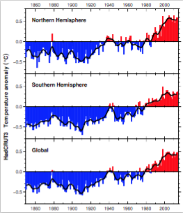
CRUTEM3 and HadCRUT3 have now been fully superseded by CRUTEM4 and HadCRUT4 (available here) and are provided here as an archive. The graphs show HadCRUT3 data up to May 2014 and links to the final data files are provided below.

The datasets have been developed in conjunction with Hadley Centre of the UK Met Office. Hemispheric and global averages as monthly and annual values are available as separate files.

This text gives some brief information for users about the datasets including:

• Scientific papers that should be consulted for complete details and referenced if any of the datasets are used
• Dataset terminology, file formats and downloads available
• Station data used for generating CRUTEM3, and a discussion of data availability issues relevant in 2008.
• Answers to some frequently-asked questions
• See also

The earlier versions (HadCRUT2 and CRUTEM2 and their variance adjusted versions) can be found here. They are no longer being updated.

References

• Brohan, P., J.J. Kennedy, I. Harris, S.F.B. Tett and P.D. Jones, 2006: Uncertainty estimates in regional and global observed temperature changes: a new dataset from 1850. J. Geophysical Research 111, D12106, doi:10.1029/2005JD006548 -- Available as PDF
• Jones, P.D., New, M., Parker, D.E., Martin, S. and Rigor, I.G., 1999: Surface air temperature and its variations over the last 150 years. Reviews of Geophysics 37, 173-199.
• Jones, P.D., Lister, D.H., Osborn, T.J., Harpham, C., Salmon, M. and Morice, C.P., 2012: Hemispheric and large-scale land surface air temperature variations: an extensive revision and an update to 2010. Journal of Geophysical Research, doi:10.1029/2011JD017139.
• Rayner, N.A., P. Brohan, D.E. Parker, C.K. Folland, J.J. Kennedy, M. Vanicek, T. Ansell and S.F.B. Tett, 2006: Improved analyses of changes and uncertainties in marine temperature measured in situ since the mid-nineteenth century: the HadSST2 dataset. J. Climate, 19, 446-469.
• Rayner, N.A., Parker, D.E., Horton, E.B., Folland, C.K., Alexander, L.V, Rowell, D.P., Kent, E.C. and Kaplan, A., 2003: Globally complete analyses of sea surface temperature, sea ice and night marine air temperature, 1871-2000. J. Geophysical Research 108, 4407, doi:10.1029/2002JD002670

CRUTEM3, CRUTEM3v, HadCRUT3, HadCRUT3v, Absolute ASCII file format
for year = 1850 to endyear for month = 1 to 12 (or less in endyear) format(2i6) year, month for row = 1 to 36 (85-90N,80-85N,75-70N,...75-80S,80-85S,85-90S) format(72(e10.3,1x)) 180W-175W,175W-170W,...,175-180E
Data represent temperature anomalies wrt 1961-90 °C Missing values represented by -1.000e+30 Absolute is just the twelve monthly averages for 1961-90: there are no years

HadSST2 ASCII file format
for year = 1850 to endyear for month = 1 to 12 (or less in endyear) format(2i12) month, year for row = 1 to 36 (85-90N,80-85N,75-70N,...75-80S,80-85S,85-90S) format(72(f7.2,1x)) 180W-175W,175W-170W,...,175-180E
Data represent temperature anomalies wrt 1961-90 °C Missing values represented by -99.99

Hemispheric/global average data file format
for year = 1850 to endyear format(i5,13f7.3) year, 12 * monthly values, annual value format(i5,12i7) year, 12 * percentage coverage of hemisphere or globe
Coverage of 0 means data not yet available

NetCDF format is read by many commercial data-processing packages (eg. IDL) and public-domain software (eg. ncview, a NetCDF viewer, and NCL, a scriptable data-manipulation and visualisation package)

Data for Downloading

Note that the end month for the hemispheric and global means is the same as for the netCDF full grid (the zipped ASCII full grid files ended earlier, as indicated below)

What are the basic raw data used?

Over land regions of the world over 3000 monthly station temperature time series are used. Coverage is denser over the more populated parts of the world, particularly, the United States, southern Canada, Europe and Japan. Coverage is sparsest over the interior of the South American and African continents and over the Antarctic. The number of available stations was small during the 1850s, but increases to over 3000 stations during the 1951-90 period. For marine regions sea surface temperature (SST) measurements taken on board merchant and some naval vessels are used. As the majority come from the voluntary observing fleet, coverage is reduced away from the main shipping lanes and is minimal over the Southern Oceans. Maps/tables giving the density of coverage through time are given for land regions by Jones and Moberg (2003) and for the oceans by Rayner et al. (2003). Both these sources also extensively discuss the issue of consistency and homogeneity of the measurements through time and the steps that have made to ensure all non-climatic inhomogeneities have been removed.

Why are sea surface temperatures rather than air temperatures used over the oceans?

Over the ocean areas the most plentiful and most consistent measurements of temperature have been taken of the sea surface. Marine air temperatures (MAT) are also taken and would, ideally, be preferable when combining with land temperatures, but they involve more complex problems with homogeneity than SSTs (Rayner et al., 2003). The problems are reduced using night only marine air temperature (NMAT) but at the expense of discarding approximately half the MAT data. Our use of SST anomalies implies that we are tacitly assuming that the anomalies of SST are in agreement with those of MAT. Many tests show that NMAT anomalies agree well with SST anomalies on seasonal and longer time scales in most open ocean areas. Globally the agreement is currently very good (Rayner et al, 2003), even better than in Folland et al. (2001b). However, some regional discrepancies in open ocean trends have recently been found in the tropics (Christy et al., 2001).

Why are the temperatures expressed as anomalies from 1961-90?

Stations on land are at different elevations, and different countries estimate average monthly temperatures using different methods and formulae. To avoid biases that could result from these problems, monthly average temperatures are reduced to anomalies from the period with best coverage (1961-90). For stations to be used, an estimate of the base period average must be calculated. Because many stations do not have complete records for the 1961-90 period several methods have been developed to estimate 1961-90 averages from neighbouring records or using other sources of data. Over the oceans, where observations are generally made from mobile platforms, it is impossible to assemble long series of actual temperatures for fixed points. However it is possible to interpolate historical data to create spatially complete reference climatologies (averages for 1961-90) so that individual observations can be compared with a local normal for the given day of the year.

Why do anomalies not average exactly zero over 1961-90?

Over both the land and marine domains considerable care has been taken in calculating the base period values for the 1961-90 period. However, as all regions don't have complete data for this 30-year period, the anomaly data do not average exactly to zero for this 30-year period. This also applies to the global and hemispheric average series as well as the individual grid-box series. However, the IPCC optimally averaged global and hemispheric time series (see later web address) are constrained to have anomalies that average to zero over 1961-90.

How are the land and marine data combined?

Both the component parts (land and marine) are separately interpolated to the same 5° x 5° latitude/longitude grid boxes. The combined versions (HadCRUT3 and HadCRUT3v) take values from each component and weight the grid boxes where both occur (coastlines and islands). The weighting method is described in Brohan et al. (2006) and is based on the size of the errors estimated for the land and marine data values.

How accurate are the hemispheric and global averages?

Annual values are approximately accurate to +/- 0.05°C (two standard errors) for the period since 1951. They are about four times as uncertain during the 1850s, with the accuracy improving gradually between 1860 and 1950 except for temporary deteriorations during data-sparse, wartime intervals. Estimating accuracy is a far from a trivial task as the individual grid-boxes are not independent of each other and the accuracy of each grid-box time series varies through time (although the variance adjustment has reduced this influence to a large extent). The issue is discussed extensively by Folland et al. (2001a,b) and Jones et al. (1997). Both Folland et al. (2001a,b) references extend discussion to the estimate of accuracy of trends in the global and hemispheric series, including the additional uncertainties related to homogeneity corrections.

In the hemispheric files averages are now given to a precision of three decimal places to enable seasonal values to be calculated to ±0.01°C. The extra precision implies no greater accuracy than two decimal places.

Why do global and hemispheric temperature anomalies differ from those quoted in the IPCC assessment and the media?

We have areally averaged grid-box temperature anomalies (using the HadCRUT3v dataset), with weighting according to the area of each 5° x 5° grid box, into hemispheric values; we then averaged these two values to create the global-average anomaly. However, the global and hemispheric anomalies used by IPCC and in the World Meteorological Organization and Met Office news releases were calculated using optimal averaging. This technique uses information on how temperatures at each location co-vary, to weight the data to take best account of areas where there are no observations at a given time. The method uses the same basic information (i.e. in future HadCRUT3v and subsequent improvements), along with the data-coverage and the measurement and sampling errors, to estimate uncertainties on the global and hemispheric average anomalies. Our alternative technique (used here) produces no estimates of uncertainties, but our results generally lie within the ranges estimated by optimum averaging. The constraint that the average be zero over 1961-90 in the optimal averages also adds a small offset compared to the other data described here.

The present optimal averages with annual uncertainties are accessible from the Hadley Centre. The data include values filtered to show decadal and longer-term variations and uncertainties. This replaces the IPCC 2001 version at the above site (see Parker et al. 2004). All other versions of global and hemispheric temperature anomalies are only steps to the IPCC series.

Why are values slightly different when I download an updated file a year later?

All the files on this page (except Absolute) will be updated on a monthly basis to include the latest month within about four weeks of its completion. Updating includes not just data for the last month but the addition of any late reports for up to approximately the last two years. In addition to this the method of variance adjustment (used for CRUTEM3v and HadCRUT3v) works on the anomalous temperatures relative to the underlying trend on an approximate 30-year timescale. With the addition of subsequent years, the underlying trend will alter slightly, changing the variance-adjusted values. Effects will be greatest on the last year of the record, but an influence can be evident for the last three to four years. Full details of the variance adjustment procedure are given in Jones et al. (2001). Approximately yearly, the optimally averaged values will also be updated to take account of such additional past information.

See also

• CRU Information Sheet no. 1: Global Temperature Record
• The previous versions of these datasets are archived:
  • HadCRUT2, CRUTEM2 and related datasets
  • HadCRUT, CRUTEM1 and related datasets
• Land Stations used by the Climatic Research Unit within CRUTEM3
• Farmer et al. 1989, "Documenting and explaining recent global-mean temperature changes" (17MB) - final report to NERC contract GR3/6565.
• Todd Mitchell at JISAO also provides a NetCDF version of Land/Ocean grid.
• Examples plots of CRU data using NCAR Command Language (NCL)

These datasets are made available under the Open Database License. Any rights in individual contents of the datasets are licensed under the Database Contents License under the conditions of Attribution and Share-Alike. Please use the attribution Climatic Research Unit, University of East Anglia